Modeling time trends for disease monitoring studies
Donegan, Connor, Amy E Hughes and Simon J Craddock Lee (2022). Colorectal Cancer Incidence, Inequalities, and Prevention Priorities in Urban Texas: Surveillance Study with the "surveil" software package. JMIR Public Health & Surveillance 8, no. 8: e34589 DOI:10.2196/34589
Software documentation: connordonegan.github.io/surveil
This paper introduces my 'surveil' R package for disease surveillance research and illustrates some advantages for health inequality research. The software provides time series models for routine public health surveillance tasks; namely, modeling time trends in mortality or disease incidence rates to make inferences about levels of risk, cumulative and period percent change, age-standardized rates, and health inequalities. Among my motivations for developing the software was to provide an accessible alternative to join-point regression, which is a standard method in cancer prevention research. The advantages over join-point include the use direct (rather than indirect) age-standardization, absence of the strict linear-trend assumption, more appropriate measures of uncertainty, and the ability to make inferences about all sorts of derivative quantities of interest including change over time as well as measures of health difference and inequality.
Because the software is designed for one very specific task, one can get started using 'surveil' with minimal R programming skills. If you download disease or mortality data from the CDC Wonder database, you'll find that the file is automatically in the correct format to start modeling with 'surveil'.
The models implemented in 'surveil' have two components or levels: first is a Poisson or binomial model or likelihood for the number of cases (deaths or disease incidence), accounting for chance variation around the trend-level of risk; the second component is a model for the trend in the level of risk. The trend models are known variably as the random-walk, first difference, or intrinsic autoregressive model. All of the model parameters also have prior distributions, which are designed to be uninformative for most use cases.
To illustrate, consider some data on colorectal cancer incidence downloaded from CRC Wonder for various age groups in Texas. The top of the file looks like this:
Table 1: Glimpse of CDC Wonder data on colorectal cancer incidence, Texas 1999-2020.
| Year | Age.Groups | Count | Population |
|---|---|---|---|
| 1999 | 45-49 | 418 | 1374078 |
| 1999 | 50-54 | 598 | 1146781 |
| 1999 | 55-59 | 728 | 863292 |
If this file were loaded into an R session as a data.frame named dat, the following code would produce a fitted model with time trends for each age group:
fit = stan_rw(dat, time = Year, group = Age.Groups)
The function expects the case counts to be stored in the column named “Count” and the population count to be found in a column named “Population” (matching the CDC Wonder data export format). The time = Year argument tells it to find the time variable in the column named ‘Year’. The group = Age.Groups' tell the software to produce separate models for each age group. (If there were just a single age group in the data, then we would simply omit the group argument.)
With one more line of code we have a publication-quality figure showing trends in CRC incidence per 100,000 at risk by age group:
plot(fit, scale = 100e3)
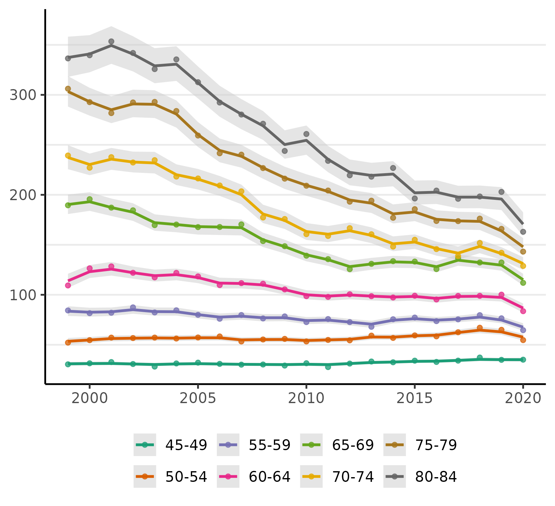
As one might expect, there has been a steep decline in CRC incidence among those of screening-age (50-75+) and, unfortunately, what may be a slow increase at younger ages (an increase which is now quite widely documented). Notably, almost all of the decline is happening at ages over 60 and especially 64. Even ages 80-84 show a very steep decline, which we might reasonably speculate is a result of (a) people choosing to continue CRC screening past the age of 75 and/or (b) that the preventive benefits of colonoscopy last about a decade (per official screening guidelines).
These age-specific trends can be summarized by percent change annually and cumulatively. The latter (cumulative percent change) is usually a more effective summary statistic because an inference about annual percent change is subject to a higher level of uncertainty. The following two lines of code will use the fitted models to produce cumulative percent change plots for each age group:
fit_pc <- apc(fit)
plot(fit_pc, cumulative = TRUE)
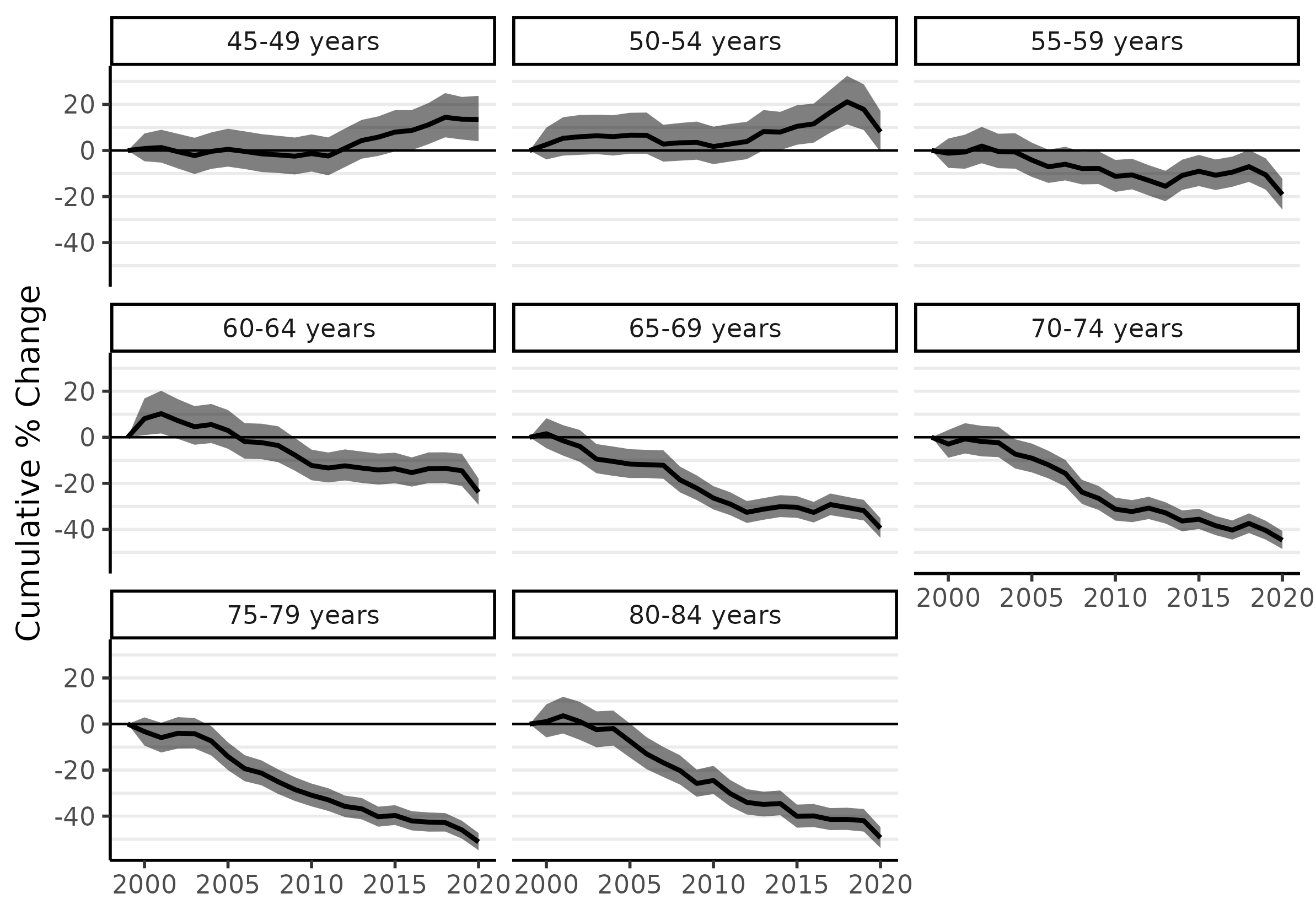
Because the pandemic interrupted a lot of cancer screening activity in 2020 (which may have resulted in cancer diagnoses being delayed to subsequent years), the estimates for 2019 are more relevant for an assessment for longer-term trends. Ages 45-49 and 50-54 increased by 13.6% and 17.8%, respectively, between 1999 and 2019. Almost all of that increase occurred since about 2012. The greatest declines occurred for the highest age groups: about 46% for ages 75-79 and 42% for ages 80-84, which is equivalent to an average of just over 2% per year since 1999.
Table 2: Cumulative % change in CRC incidence, 1999 to 2019.
| Age Group | Cum. % change | 95% cred. interval |
|---|---|---|
| 45-49 | 13.6 | 4.8, 23.3 |
| 50-54 | 17.8 | 8.9, 29.0 |
| 55-59 | -10.6 | -17, -3.4 |
| 60-64 | -14.5 | -21.2, -7.2 |
| 65-69 | -31.9 | -36.1, -27.2 |
| 70-74 | -40.5 | -44.4, -36.3 |
| 75-79 | -46 | -49.8, -42.0 |
| 80-84 | -42 | -46.7, -37.0 |
Returning to the R code, the data in Table 2 can be found by printing the cpc slot in the fit_pc object (this will show a summary of CPC estimates for all years and age groups):
print( fit_pc$cpc )
An advantage of ‘surveil’ is that users can calculate any kind of summary statistic they like and obtain appropriate credible intervals for them, such as percent change between any two years or a rate ratio for two groups. More background and examples can be found in the ‘surveil’ vignette on MCMC analysis with surveil. A particularly important example is direct age-standardization.
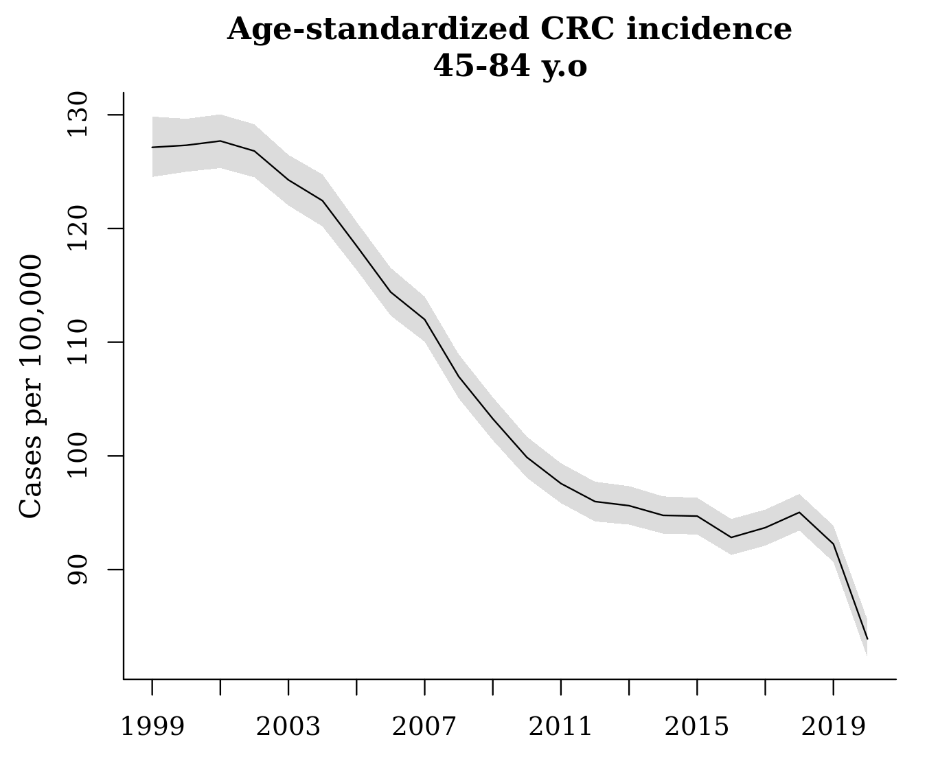
‘surveil’ comes packaged with the 2000 U.S. standard million population, we can be loaded by entering data(standard). To apply direct age standardization to our model of age-specific rates we pass our model and the standard population data to the standardize function, as follows:
data(standard)
fit_st <- standardize(fit, label = standard$age, standard_pop = standard$standard_pop)
The output, fit_st, can be treated just like the other ‘surveil’ model - we can produce a nice plot of age-standardized rates using plot(fit_st, scale = 100e3) or we can use the summary data in the output to create a custom plot (as in Fig. 3). As noted above, the sharp decline in 2020 is likely due only to pandemic restrictions that prevented people from receiving early diagnoses.
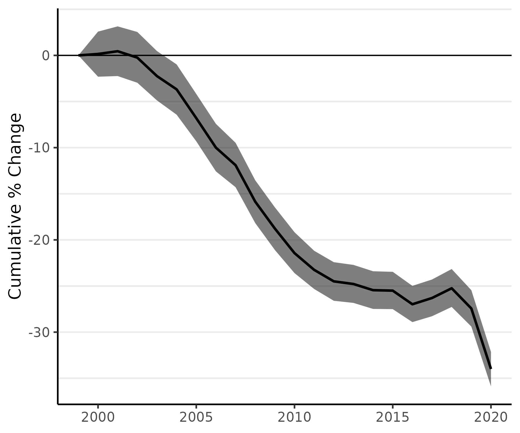
As our final step here, we can also apply our percent change methods to the age-standardized model, fit_st, and then plot the cumulative percent change in age-standardized rates:
fit_st_pc <- apc(fit_st)
plot(fit_st_pc, cum = TRUE)
If you want to follow this example on your computer, you can use the following R code:
# install surveil (if necessary)
if (!require("surveil")) install.packages("surveil")

# load the package
library(surveil)

# data source
crc_url <- "https://raw.githubusercontent.com/ConnorDonegan/connordonegan.github.io/main/assets/00-CDCWonder-crc-45-84.txt"

# read the data into R
dat <- read.table(crc_url, header = TRUE, sep = "\t")

# fit Poisson random walk models by age group
fit = stan_rw(dat, time = Year, group = Age.Groups)

# same as obove but with parallel processing (faster)
fit = stan_rw(dat, time = Year, group = Age.Groups.Code, cores = 4)

# plot time trends (per 100,000)
plot(fit, scale = 100e3)

# calculate percent change
fit_pc <- apc(fit)

# plot cumulative percent change
plot(fit_pc, cumulative = TRUE)

# print cumulative percent change
print(fit_pc$cpc)

# age-standardized rates
data(standard)
fit_st <- standardize(fit, label = standard$age, standard_pop = standard$standard_pop)

# plot age standardized rates
plot(fit_st, scale = 100e3)

# plot cumulative % change in age standardized rates
fit_st_pc <- apc(fit_st)
plot(fit_st_pc, cum = TRUE)

# custom plot with base R graphics
stand_df <- fit_st$standard_summary
attach(stand_df)
ogpar <- par(family = "Serif",
    mar = c(3, 4, 3, 1))
plot(c(time_label, time_label),
     c(.lower * 100e3, .upper * 100e3),
     t = 'n',
     main = "Age-standardized CRC incidence\n45-84 y.o",
     axes = FALSE,
     xlab = NA,
     ylab = NA)
polygon(c(time_label, rev(time_label)),
        c(.lower * 100e3, rev(.upper * 100e3)),
        col = rgb(.1, .1, .1, .15), border = 2,
        lwd = 2, lty = 0)
axis(2, at = seq(0, 200, by = 10))
axis(1, at = seq(1997, 2021, by = 2))
lines(time_label, stand_rate * 100e3)
mtext("Cases per 100,000", side = 2, line = 2.5, col = 1, cex = 1.1)
detach(stand_df)

# reset graphics parameters
par(ogpar)