This vignette describes the method of direct age-standardization (Broemeling 2020) and then demonstrates implementation with surveil.
Data
The demonstration will use age-specific cancer incidence for the entire population of the United States of America, 1999-2017.
library(surveil)
data(cancer)
head(cancer)
#>   Year   Age Count Population
#> 1 1999    <1   866    3708753
#> 2 1999   1-4  2959   14991152
#> 3 1999   5-9  2226   20146188
#> 4 1999 10-14  2447   19742631
#> 5 1999 15-19  3875   19585857
#> 6 1999 20-24  5969   18148795
We will also use the age distribution of the United States in the year 2000 (2000 U.S. standard million population, see ?standard):
data(standard)
print(standard)
#>    age.id   age standard_pop
#> 1       1    <1        13818
#> 2       2   1-4        55317
#> 3       3   5-9        72533
#> 4       4 10-14        73032
#> 5       5 15-19        72169
#> 6       6 20-24        66478
#> 7       7 25-29        64529
#> 8       8 30-34        71044
#> 9       9 35-39        80762
#> 10     10 40-44        81851
#> 11     11 45-49        72118
#> 12     12 50-54        62716
#> 13     13 55-59        48454
#> 14     14 60-64        38793
#> 15     15 65-69        34264
#> 16     16 70-74        31773
#> 17     17 75-79        26999
#> 18     18 80-84        17842
#> 19     19   85+        15508
Notice that the five-year age groups in the cancer data match the age groups provided by standard.
In some cases, one is only interested in a subset of age groups. For the following examples, we will limit the analysis to persons 50-69 years old:
cancer2 <- subset(cancer, grepl("50-54|55-59|60-64|65-69", Age))
head(cancer2)
#>    Year   Age  Count Population
#> 12 1999 50-54  99571   16557188
#> 13 1999 55-59 121501   12787366
#> 14 1999 60-64 143968   10435791
#> 15 1999 65-69 178278    9311622
#> 31 2000 50-54 106458   17394053
#> 32 2000 55-59 127276   13258779
Subsetting the data allows for faster results. If instead of making this selection we were to use the entire age distribution in our analysis, all of the following discussion and code could still proceed unchanged.
Direct age-standardization
Let \(\theta_i\) be the disease risk in the \(i^{th}\) age group, and let \(\omega_i\) be the standard population count for that age group. Then the age-standardized risk is: \[SR = \frac{\sum_i \theta_i \omega_i}{\sum_i \omega_i}\] That is, age-standardization consists of multiplying actual age-specific rates by false, but fixed, population sizes. This enables comparisons to be made across populations that have different age structures.
There are two steps to producing age-standardized rates using surveil:
- Model time trends for each age group using
stan_rw. - Convert the age-specific model results into age-standardized rates using the
standardizefunction.
Modeling age-specific risk
To model age-specific rates, provide the stan_rw function with the cancer data and tell it which column contains the time period indicator (Year) and which column contains the grouping variable (Age):
fit <- stan_rw(cancer2, time = Year, group = Age,
               refresh = 0,# silences some printing
               iter = 2e3,
               chains = 2) # for demo speed only. Use the default chains = 4
#> Distribution: normal
#> Distribution: normal
#> Warning: The largest R-hat is 1.06, indicating chains have not mixed.
#> Running the chains for more iterations may help. See
#> https://mc-stan.org/misc/warnings.html#r-hat
#> Warning: Bulk Effective Samples Size (ESS) is too low, indicating posterior means and medians may be unreliable.
#> Running the chains for more iterations may help. See
#> https://mc-stan.org/misc/warnings.html#bulk-ess
#> [1] "Setting normal prior(s) for eta_1: "
#>  location scale
#>        -6     5
#> [1] "\nSetting half-normal prior for sigma: "
#>  location scale
#>         0     1
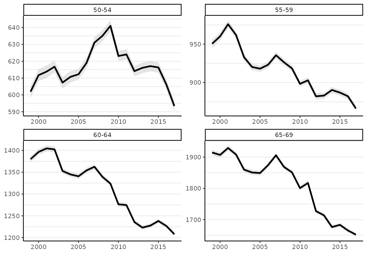
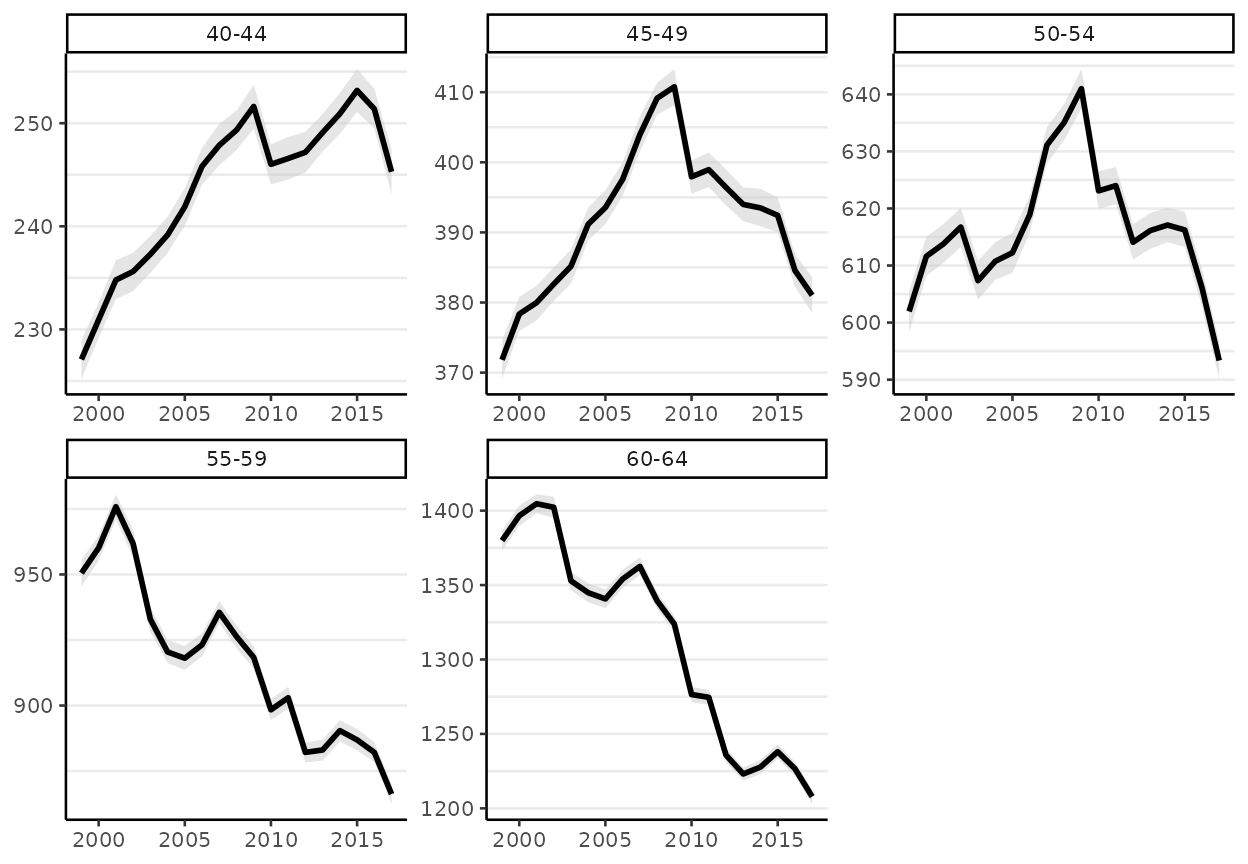
The default plot method will return all of the age-specific time trends on the same plot. It is sometimes easier to understand the results using a grid of multiple small plots (facet = TRUE). There is also an option to allow the scale of the y-axes to adjust for each age group (facet_scales = "free"):
plot(fit,
     facet = TRUE,          # plot small multiples
     facet_scales = "free", # y-axes vary across plots
     base_size = 10,      # control text size
     size = 0,            # removes crude rates from the plots
     scale = 100e3        # plot rates per 100,000
     )
#> Plotted rates are per 100,000
The figures contain estimates with shaded 95% credible intervals.
In addition to examining trends in age-specific rates (as above), we can also convert each age-specific trend to its annual percent change or cumulative percent change.

Age-standardizing model results
The standardize function takes a fitted model, plus the standard population, and returns standardized rates (SRs):
fit_sr <- standardize(fit,
                        label = standard$age,
                        standard_pop = standard$standard_pop)
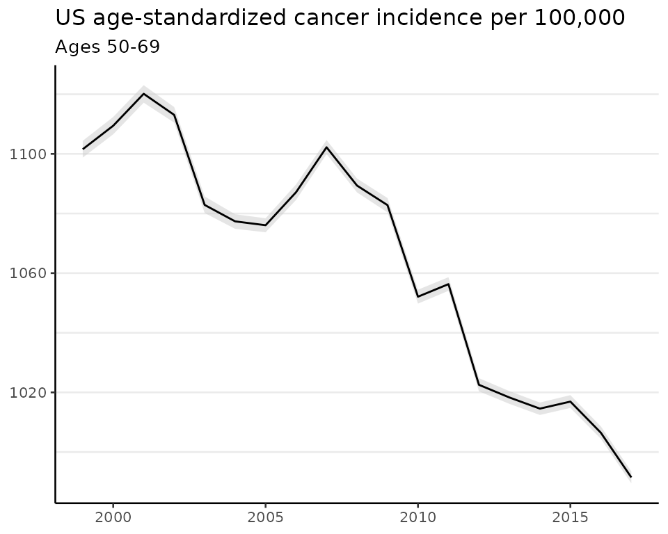
As usual, surveil provides a plotting method for the fit_sr object:
# load ggplot2 to enable additional plot customization
library(ggplot2)
plot(fit_sr, scale = 100e3, base_size = 10) +
  labs(title = "US age-standardized cancer incidence per 100,000",
  subtitle = "Ages 50-69")
#> Plotted rates are per 100,000
as well as a printing method:
print(fit_sr, scale = 100e3)
#> Summary of age-standardized surveil model results
#> As rate per 100,000 at risk
#> Time periods: 19
#>  time_label stand_rate .lower .upper
#>        1999       1102   1099   1104
#>        2000       1109   1107   1112
#>        2001       1120   1117   1123
#>        2002       1113   1110   1116
#>        2003       1083   1080   1086
#>        2004       1077   1075   1080
#>        2005       1076   1074   1078
#>        2006       1087   1085   1090
#>        2007       1102   1100   1105
#>        2008       1089   1087   1092
#>        2009       1083   1080   1085
#>        2010       1052   1050   1054
#>        2011       1056   1054   1059
#>        2012       1023   1020   1025
#>        2013       1018   1016   1020
#>        2014       1015   1012   1017
#>        2015       1017   1015   1019
#>        2016       1006   1004   1009
#>        2017        991    990    993
To learn about the contents of fit_sr, see ?standardize or explores its contents as you would a list using names(fit_sr), fit_sr$standard_summary, head(fit_sr$standard_samples), etc.
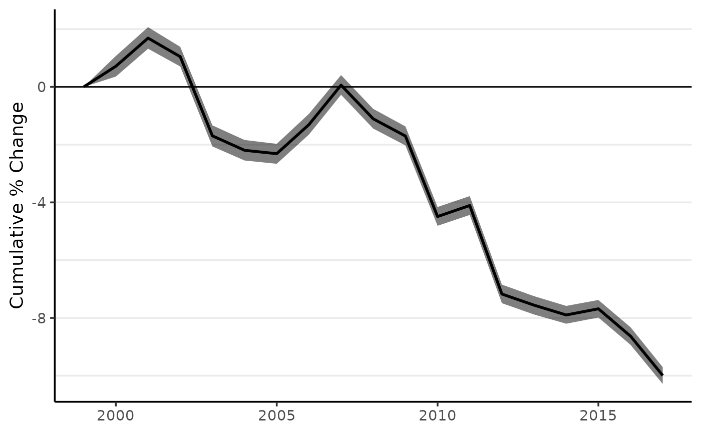
The apc function and its methods for printing and plotting can be applied to the age-standardized results:
fit_sr_pc <- apc(fit_sr)
plot(fit_sr_pc, cum = TRUE)
References
Broemeling, Lyle D. 2020. Bayesian Methods in Epidemiolgy. CRC Press.
Donegan, Connor, Amy E. Hughes, and Simon J. Craddock Lee. 2022. “Colorectal Cancer Incidence, Inequality, and Prevention Priorities in Urban Texas: Surveillance Study with the ‘Surveil’ Software Pakcage.” JMIR Public Health & Surveillance 8 (8): e34589. https://doi.org/10.2196/34589.